
This article is part of the Circuits thread, a collection of short articles and commentary by an open scientific collaboration delving into the inner workings of neural networks.
The first few articles of the Circuits project will be focused on early vision in InceptionV1
Over the course of these layers, we see the network go from raw pixels up to sophisticated boundary detection, basic shape detection (eg. curves, circles, spirals, triangles), eye detectors, and even crude detectors for very small heads. Along the way, we see a variety of interesting intermediate features, including Complex Gabor detectors (similar to some classic “complex cells” of neuroscience), black and white vs color detectors, and small circle formation from curves.
Studying early vision has two major advantages as a starting point in our investigation.
Firstly, it’s particularly easy to study:
it’s close to the input, the circuits are only a few layers deep, there aren’t that many different neurons,
Before we dive into detailed explorations of different parts of early vision, we wanted to give a broader overview of how we presently understand it. This article sketches out our understanding, as an annotated collection of what we call “neuron groups.” We also provide illustrations of selected circuits at each layer.
By limiting ourselves to early vision, this article “only” considers the first 1,056 neurons of InceptionV1.
Playing Cards with Neurons
Dmitri Mendeleev is often accounted to have discovered the Periodic Table by playing “chemical solitaire,” writing the details of each element on a card and patiently fiddling with different ways of classifying and organizing them. Some modern historians are skeptical about the cards, but Mendeleev’s story is a compelling demonstration of that there can be a lot of value in simply organizing phenomena, even when you don’t have a theory or firm justification for that organization yet. Mendeleev is far from unique in this. For example, in biology, taxonomies of species preceded genetics and the theory of evolution giving them a theoretical foundation.
Our experience is that many neurons in vision models seem to fall into families of similar features. For example, it’s not unusual to see a dozen neurons detecting the same feature in different orientations or colors. Perhaps even more strikingly, the same “neuron families” seem to recur across models! Of course, it’s well known that Gabor filters and color contrast detectors reliably comprise neurons in the first layer of convolutional neural networks, but we were quite surprised to see this generalize to later layers.
This article shares our working categorization of units in the first five layers of InceptionV1 into neuron families. These families are ad-hoc, human defined collections of features that seem to be similar in some way. We’ve found these helpful for communicating among ourselves and breaking the problem of understanding InceptionV1 into smaller chunks. While there are some families we suspect are “real”, many others are categories of convenience, or categories we have low-confidence about. The main goal of these families is to help researchers orient themselves.
In constructing this categorization, our understanding of individual neurons was developed by looking at feature visualizations, dataset examples, how a feature is built from the previous layer, how it is used by the next layer, and other analysis. It’s worth noting that the level of attention we’ve given to individual neurons varies greatly: we’ve dedicated entire forthcoming articles to detailed analysis some of these units, while many others have only received a few minutes of cursory investigation.
In some ways, our categorization of units is similar to Net Dissect mixed3b we see many units which appear from dataset examples likely to be familiar feature types like curve detectors, divot detectors, boundary detectors, eye detector, and so forth, but are classified as weakly correlated with another feature — often objects that it seems unlikely could be detected at such an early layer.
Or in another fun case, there is a feature (372) which is most correlated with a cat detector, but appears to be detecting left-oriented whiskers!
Caveats
- This is a broad overview and our understanding of many of these units is low-confidence. We fully expect, in retrospect, to realize we misunderstood some units and categories.
- Many neuron groups are catch-all categories or convenient organizational categories that we don’t think reflect fundamental structure.
- Even for neuron groups we suspect do reflect a fundamental structure (eg. some can be recovered from factorizing the layer’s weight matrices) the boundaries of these groups can be blurry and some neurons inclusion involve judgement calls.
Presentation of Neurons
In order to talk about neurons, we need to somehow represent them.
While we could use neuron indices, it’s very hard to keep hundreds of numbers straight in one’s head.
Instead, we use feature visualizations
When we represent a neuron with a feature visualization, we don’t intend to claim that the feature visualization captures the entirety of the neuron’s behavior.
Rather, the role of a feature visualization is like a variable name in understanding a program.
It replaces an arbitrary number with a more meaningful symbol
Presentation of Circuits
Although this article is focused on giving an overview of the features which exist in early vision, we’re also interested in understanding how they’re computed from earlier features.
To do this, we present circuits consisting of a neuron, the units it has the strongest (L2 norm) weights to in the previous layer, and the weights between them.mixed3a and mixed3b are in branches consisting of a “bottleneck” 1x1 conv that greatly reduces the number of channels followed by a 5x5 conv. Although there is a ReLU between them, we generally think of them as a low rank factorization of a single weight matrix and visualize the product of the two weights. Additionally, some neurons in these layers are in a branch consisting of maxpooling followed by a 1x1 conv; we present these units as their weights replicated over the region of their maxpooling.
For example, here is a circuit of a circle detecting unit in mixed3a being assembled from earlier curves and a primitive circle detector.
We’ll discuss this example in more depth later.
At any point, you can click on a neuron’s feature visualization to see its weights to the 50 neurons in the previous layer it is most connected to (that is, how it assembled from the previous layer, and also the 50 neurons in the next layer it is most connected to (that is, how it is used going forward). This allows further investigation, and gives you an unbiased view of the weights if you’re concerned about cherry-picking.
conv2d0
The first conv layer of every vision model we’ve looked at is mostly comprised of two kinds of features: color-contrast detectors and Gabor filters.
InceptionV1′s conv2d0 is no exception to this rule, and most of its units fall into these categories.
In contrast to other models, however, the features aren’t perfect color contrast detectors and Gabor filters.
For lack of a better word, they’re messy.
We have no way of knowing, but it seems likely this is a result of the gradient not reaching the early layers very well during training.
Note that InceptionV1 predated the adoption of modern techniques like batch norm and Adam, which make it much easier to train deep models well.
If we compare to the TF-Slim
One subtlety that’s worth noting here is that Gabor filters almost always come in pairs of weights which are negative versions of each other, both in InceptionV1 and other vision models. A single Gabor filter can only detect edges at some offsets, but the negative version fills in holes, allowing for the formation of complex Gabor filters in the next layer.
Gabor Filters 44%

9

53

54

15

22

39

30

1

3

49

14

17

62

20

27

0

10

28

21

63

45

18

6

57

41

43

46

8
Show all 28 neurons.
Collapse neurons.
Gabor filters are a simple edge detector, highly sensitive to the alignment of the edge. They’re almost universally found in the fist layer of vision models. Note that Gabor filters almost always come in pairs of negative reciprocals.
Color Contrast 42%

59

23

5

7

48

29

12

24

55

13

32

50

36

37

16

11

33

34

47

38

58

2

60

61

4

51

25
Show all 27 neurons.
Collapse neurons.


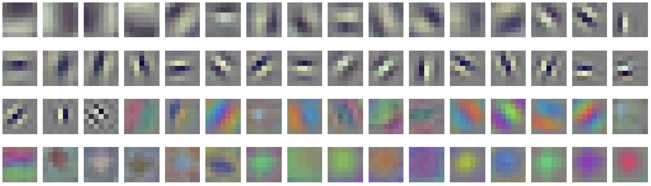
conv2d1
In conv2d1, we begin to see some of the classic complex cell features of visual neuroscience.
These neurons respond to similar patterns to units in conv2d0, but are invariant to some changes in position and orientation.
Complex Gabors: A nice example of this is the “Complex Gabor” feature family. Like simple Gabor filters, complex Gabors detect edges. But unlike simple Gabors, they are relatively invariant to the exact position of the edge or which side is dark or light. This is achieved by being excited by multiple Gabor filters in similar orientations — and most critically, by being excited by “reciprocal Gabor filters” that detect the same pattern with dark and light switched. This can be seen as an early example of the “union over cases” motif.
Note that conv2d1 is a 1x1 convolution, so there’s only a single weight — a single line, in this diagram — between each channel in the previous and this one.
In addition to Complex Gabors, we see a variety of other features, including more invariant color contrast detectors, Gabor-like features that are less selective for a single orientation, and lower-frequency features.
Low Frequency 27%

1

13

27

47

56

60

23

49

0

43

28

29

34

8

37

19

15
Show all 17 neurons.
Collapse neurons.
These units seem to respond to lower-frequency edge patterns, but we haven’t studied them very carefully.
Gabor Like 17%

4

6

32

38

41

63

7

11

18

24

39
Show all 11 neurons.
Collapse neurons.
These units respond to edges stimuli, but seem to respond to a wider range of orientations, and also respond to color contrasts that align with the edge. We haven’t studied them very carefully.
Color Contrast 16%

5

9

10

12

20

21

42

45

50

53
These units detect a color on one side of the receptive field, and a different color on the opposite side. Composed of lower-level color contrast detectors, they often respond to color transitions in a range of translation and orientation variations. Compare to earlier color contrast (
conv2d0) and later color contrast (conv2d2, mixed3a, mixed3b).Multicolor 14%

3

33

35

40

17

16

57

26

31
These units respond to mixtures of colors without an obvious strong spatial structure preference.
Complex Gabor 14%

51

58

30

25

52

54

22

61

55
Like Gabor Filters, but fairly invariant to the exact position, formed by adding together multiple Gabor detectors in the same orientation but different phases. We call these ‘Complex’ after complex cells in neuroscience.
Color 6%

2

48

36

46
Two of these units seem to track brightness (bright vs dark), while the other two units seem to mostly track hue, dividing the space of hues between them. One responds to red/orange/yellow, while the other responds to purple/blue/turqoise. Unfortunately, their circuits seem to heavily rely on the existence of a Local Response Normalization layer after
conv2d0, which makes it hard to reason about.


hatch 2%

14
This unit detects Gabor patterns in two orthogonal directions, selecting for a “hatch” pattern.
conv2d2
In conv2d2 we see the emergence of very simple shape predecessors.
This layer sees the first units that might be described as “line detectors”, preferring a single longer line to a Gabor pattern and accounting for about 25% of units.
We also see tiny curve detectors, corner detectors, divergence detectors, and a single very tiny circle detector.
One fun aspect of these features is that you can see that they are assembled from Gabor detectors in the feature visualizations, with curves being built from small piecewise Gabor segments.
All of these units still moderately fire in response to incomplete versions of their feature, such as a small curve running tangent to the edge detector.
Since conv2d2 is a 3x3 convolution, our understanding of these shape precursor features (and some texture features) maps to particular ways Gabor and lower-frequency edges are being spatially assembled into new features.
At a high-level, we see a few primary patterns:
We also begin to see various kinds of texture and color detectors start to become a major constituent of the layer, including color-contrast and color center surround features, as well as Gabor-like, hatch, low-frequency and high-frequency textures. A handful of units look for different textures on different sides of their receptive field.
Color Contrast 21%

10

36

172

56

131

176

35

41

45

126

77

120

101

0

43

62

106

169

127

6

68

60

134

51

74

85

115

24

14

16

151

168

19

7

88

177

183

76

70

122
Show all 40 neurons.
Collapse neurons.
These units detect a color on one side of the receptive field, and a different color on the opposite side. Composed of lower-level color contrast detectors, they often respond to color transitions in a range of translation and orientation variations. Compare to earlier color contrast (
conv2d0, conv2d1) and later color contrast (mixed3a, mixed3b).Line 17%

107

31

9

112

133

103

97

125

20

33

113

185

150

166

157

57

145

48

55

15

152

11

141

174

44

170

27

100

30

82

65

3

108
Show all 33 neurons.
Collapse neurons.
These units are beginning to look for a single primary line. Some look for different colors on each side. Many exhibit “combing” (small perpendicular lines along the main one), a very common but not presently understood phenomenon in line-like features across vision models. Compare to shifted lines and later lines (
mixed3a).Shifted Line 8%

116

61

8

22

69

96

78

18

17

132

190

64

81

154

179

136
Show all 16 neurons.
Collapse neurons.
These units look for edges “shifted” to the side of the receptive field instead of the middle. This may be linked to the many 1x1 convs in the next layer. Compare to lines (non-shifted) and later lines (
mixed3a).Textures 8%

21

52

59

119

148

161

162

186

189

191

72

46

67

40

38
Show all 15 neurons.
Collapse neurons.
A broad category of units detecting repeating local structure.
Other Units 7%

2

50

54

66

84

90

93

109

129

149

153

158

175

187
Show all 14 neurons.
Collapse neurons.
Catch-all category for all other units.
Color Center-Surround 7%

155

34

156

13

49

138

23

160

86

124

25

4

29
Show all 13 neurons.
Collapse neurons.
These units look for one color in the middle and another (typically opposite) on the boundary. Genereally more sensitive to the center than boundary. Compare to later Color Center-Surround (
mixed3a) and Color Center-Surround (mixed3b).Tiny Curves 6%

182

117

171

111

63

130

146

180

39

140

32

80
Show all 12 neurons.
Collapse neurons.
Very small curve (and one circle) detectors. Many of these units respond to a range of curvatures all the way from a flat line to a curve. Compare to later curves (
mixed3a) and curves (mixed3b). See also circuit example and discussion of use in forming small circles/eyes (mixed3a).Early Brightness Gradient 6%

94

142

99

104

163

188

98

165

83

79

128

5
Show all 12 neurons.
Collapse neurons.
These units detect oriented gradients in brightness. They support a variety of similar units in the next layer. Compare to later brightness gradients (
mixed3a) and brightness gradients (mixed3b).Gabor Textures 6%

89

91

110

114

123

135

139

143

144

167

173

118
Show all 12 neurons.
Collapse neurons.
Like complex Gabor units from the previous layer, but larger. They’re probably starting to be better described as a texture.
Texture Contrast 4%

1

37

71

73

105

147

178

181
These units look for different textures on opposite sides of their receptive field. One side is typically a Gabor pattern.
Hatch Textures 3%

164

184

28

121

159

102
These units detect Gabor patterns in two orthogonal directions, selecting for a “hatch” pattern.
Color/Multicolor 3%

58

75

92

42

12
Several units look for mixtures of colors but seem indifferent to their organization.
Corners 2%

47

87

95

26
These units detect two Gabor patterns which meet at apprixmately 90 degrees, causing them to respond to corners.


mixed3a
mixed3a has a significant increase in the diversity of features we observe.
Some of them — curve detectors and high-low frequency detectors — were discussed in Zoom In
and will be discussed again in later articles in great detail.
But there are some really interesting circuits in mixed3a which we haven’t discussed before,
and we’ll go through a couple selected ones to give a flavor of what happens at this layer.
Black & White Detectors: One interesting property of mixed3a is the emergence of “black and white” detectors, which detect the absence of color.
Prior to mixed3a, color contrast detectors look for transitions of a color to near complementary colors (eg. blue vs yellow).
From this layer on, however, we’ll often see color detectors which compare a color to the absence of color.
Additionally, black and white detectors can allow the detection of greyscale images, which may be correlated with ImageNet categories (see
4a:479
which detects black and white portraits).
The circuit for our black and white detector is quite simple:
almost all of its large weights are negative, detecting the absence of colors.
Roughly, it computes NOT(color_feature_1 OR color_feature_2 OR ...).
Small Circle Detector: We also see somewhat more complex shapes in mixed3a. Of course, curves (which we discussed in Zoom In) are a prominent example of this.
But there’s lots of other interesting examples.
For instance, we see a variety of small circle and eye detectors form
by piecing together early curves and circle detectors (conv2d2):
Triangle Detectors: While on the matter of basic shapes, we also see triangle detectors
form from earlier line (conv2d2) and shifted line (conv2d2) detectors.
However, in practice, these triangle detectors (and other angle units) seem to often just be used as multi-edge detectors downstream, or in conjunction with many other units to detect convex boundaries.
The selected circuits discussed above only scratch the surface of the intricate structure in mixed3a.
Below, we provide a taxonomized overview of all of them:
Texture 25%

246

242

253

232

233

209

139

65

44

51

194

207

111

218

224

225

215

198

62

21

254

255

61

2

3

8

12

53

56

102

148

244

250

11

238

248

9

219

234

252

236

5

183

241

229

93

243

99

45

33

135

231

60

235

48

55

42

151

54

72

6

239

66

129

245
Show all 65 neurons.
Collapse neurons.
This is a broad, not very well defined category for units that seem to look for simple local structures over a wide receptive field, including mixtures of colors. Many live in a branch consisting of a maxpool followed by a 1x1 conv, which structurally encourages this.Maxpool branches (ie. maxpool 5x5 stride 1 -> conv 1x1) have large receptive fields, but can’t control where in in their receptive field each feature they detect is, nor the relative position of these features. In early vision, this unstructured of feature detection makes them a good fit for textures.
Color Center-Surround 12%

119

34

167

76

19

30

131

251

226

13

7

50

1

4

41

192

36

40

103

213

10

35

221

193

158

73

74

177

97

141
Show all 30 neurons.
Collapse neurons.
These units look for one color in the center, and another (usually opposite) color surrounding it. They are typically much more sensitive to the center color than the surrounding one. In visual neuroscience, center-surround units are classically an extremely low-level feature, but we see them in the later parts of early vision. Compare to earlier Color Center-Surround (
conv2d2) and later Color Center-Surround (mixed3b).High-Low Frequency 6%

110

180

153

106

112

186

132

136

117

113

108

70

86

88

160
Show all 15 neurons.
Collapse neurons.
These units look for transitions from high-frequency texture to low-frequency. They are primarily used by boundary detectors (
A detailed article on these is forthcoming.
mixed3b) as an additional cue for a boundary between objects. (Larger scale high-low frequency detectors can be found in mixed4a (245, 93, 392, 301), but are not discussed in this article.) A detailed article on these is forthcoming.
Brightness Gradient 6%

216

127

22

182

162

25

249

15

28

59

29

196

206

18

247
Show all 15 neurons.
Collapse neurons.
These units detect brightness gradients. Among other things they will help detect specularity (shininess), curved surfaces, and the boundary of objects. Compare to earlier brightness gradients (
conv2d2) and later brightness gradients (mixed3b).Color Contrast 5%

195

84

85

123

203

217

199

211

205

212

202

200

138

32
Show all 14 neurons.
Collapse neurons.
These units look for one color on one side of their receptive field, and another (usually opposite) color on the opposing side. They typically don’t care about the exact position or orientation of the transition. Compare to earlier color contrast (
conv2d0, conv2d1, conv2d2) and later color contrast (mixed3b).Complex Center-Surround 5%

178

181

161

166

172

68

130

49

52

114

115

120

144

37
Show all 14 neurons.
Collapse neurons.
This is a broad, not very well defined category for center-surround units that detect a pattern or complex texture in their center.
Line Misc. 5%

191

121

116

14

24

0

159

152

165

83

173

87

90

82
Show all 14 neurons.
Collapse neurons.
Broad, low confidence organizational category.
Lines 5%

227

75

146

69

169

57

154

187

27

134

150

240

101

176
Show all 14 neurons.
Collapse neurons.
Units used to detect extended lines, often further excited by different colors on each side. A few are highly combed line detectors that aren’t obviously such at first glance. The decision to include a unit was often decided by whether it seems to be used by downstream client units as a line detector.
Other Units 5%

38

43

58

67

190

109

122

128

142

143

155

170

179

184
Show all 14 neurons.
Collapse neurons.
Catch-all category for all other units.
Repeating patterns 5%

237

31

17

20

39

126

124

156

98

105

230

228
Show all 12 neurons.
Collapse neurons.
This is broad, catch-all category for units that seem to look for repeating local patterns that seem more complex than textures.
Curves 4%

81

104

92

145

95

163

171

71

147

189

137
Show all 11 neurons.
Collapse neurons.
These curve detectors detect significantly larger radii curves than their predecessors. They will be refined into more specific, larger curve detectors in the next layer. Compare to earlier curves (
See the full paper on curve detectors.
conv2d2) and later curves (mixed3b). See the full paper on curve detectors.
BW vs Color 4%

214

208

201

223

210

197

222

204

220
These “black and white” detectors respond to absences of color. Prior to this, color detectors contrast to the opposite hue, but from this point on we’ll see many compare to the absence of color. See also BW circuit example and discussion.
Angles 3%

188

94

164

107

77

157

149

100
Units that detect multiple lines, forming angles, triangles and squares. They generally respond to any of the individual lines, and more strongly to them together.
Fur Precursors 3%

46

47

26

63

80

23

16
These units are not yet highly selective for fur (they also fire for other high-frequency patterns), but their primary use in the next layer is supporting fur detection. At the 224x224 image resolution, individual fur hairs are generally not detectable, but tufts of fur are. These units use Gabor textures to detect those tufts in different orientations. The also detect lower frequency edges or changes in lighting perpendicular to the tufts.
Eyes / Small Circles 2%

174

168

79

125

175
We think of eyes as high-level features, but small eye detectors actually form very early. Compare to later eye detectors (
mixed3b). See also circuit example and discussion.Crosses / Diverging Lines 2%

91

185

64

118
These units seem to respond to lines crossing or to lines diverging from a central point.


Line Ends 1%

133

96
These units detect a line ending or sharply turning. Often used in boundary detection and more complex shape detectors.
mixed3b
mixed3b straddles two levels of abstraction.
On the one hand, it has some quite sophisticated features that don’t really seem like they should be characterized as “early” or “low-level”: object boundary detectors, early head detectors, and more sophisticated part of shape detectors.
On the other hand, it also has many units that still feel quite low-level, such as color center-surround units.
Boundary detectors: One of the most striking transitions in mixed3b is the formation of boundary detectors.
When you first look at the feature visualizations and dataset examples,
you might think these are just another iteration of edge or curve detectors.
But they are in fact combining a variety of cues to detect boundaries and transitions between objects.
Perhaps the most important one is the high-low frequency detectors we saw develop at the previous layer.
Notice that it largely doesn’t care which direction the change in color or frequency is, just that there’s a change.
We sometimes find it useful to think about the “goal” of early vision.
Gradient descent will only create features if they are useful for features in later layers.
Which later features incentivized the creation of the features we see in early vision?
These boundary detectors seem to be the “goal” of the high-low frequency detectors (mixed3a) we saw in the previous layer.
Curve-based Features: Another major theme in this layer is the emergence of more complex and specific shape detectors based on curves. These include more sophisticated curves, circles, S-shapes, spirals, divots, and “evolutes” (a term we’ve repurposed to describe units detecting curves facing away from the middle). We’ll discuss these in detail in a forthcoming article on curve circuits, but they warrant mention here.
Conceptually, you can think of the weights as piecing together curve detectors as something like this:
Fur detectors: Another interesting (albeit, probably quite specific to the dog focus of ImageNet)
circuit is the implementation of “oriented fur detectors” which detect fur parting, like hair on one’s head.
They’re implemented by piecing together fur precursors (mixed3a) so that they converge in a particular way.
Again, these circuits only scratch the surface of mixed3b.
Since it’s a larger layer with lots of families, we’ll go through a couple particularly interesting and well understood families first:
Boundary 8%

220

402

364

293

356

151

203

394

376

400

328

219

320

313

329

321

251

298

257

143

366

345

405

414

301

368

398

383

396

261

184

144

360

183

239

386
Show all 36 neurons.
Collapse neurons.
These units use multiple cues to detect the boundaries of objects. They vary in orientation, detecting convex/concave/straight boundaries, and detecting artificial vs fur foregrounds. Cues they rely on include line detectors, high-low frequency detectors, and color contrast.
Proto-Head 3%

362

413

334

331

174

225

393

185

435

180

441

163
Show all 12 neurons.
Collapse neurons.
The tiny eye detectors, along with texture detectors for fur, hair and skin developed at the previous layer enable these early head detectors, which will continue to be refined in the next layer.
Generic, Oriented Fur 2%

57

387

404

333

375

381

335

378

62

52
We don’t typically think of fur as an oriented feature, but it is. These units detect fur parting in various ways, much like how hair on your head parts.
Curves 2%

379

406

385

343

342

388

340

330

349

324
The third iteration of curve detectors. They detect larger radii curves than their predecessors, and are the first to not slightly fire for curves rotated 180 degrees. Compare to the earlier curves (conv2d2) and curves (mixed3a).
See the full paper on curve detectors.
See the full paper on curve detectors.


Brightness Gradients 1%

0

317

136

455

417

469
These units detect brightness gradients. This is their third iteration; compare to earlier brightness gradients (
conv2d2) and brightness gradients (mixed3a).Eyes 1%

370

352

363

322

83

199
Again, we continue to see eye detectors quite early in vision. Note that several of these detect larger eyes than the earlier eye detectors (mixed3a). In the next layer, we see much larger scale eye detectors again.


Curve Shapes 1%

325

338

327

347
Simple shapes created by composing curves, such as spirals and S-curves.
Circles / Loops 1%

389

384

346

323
Piece together curves in a circle or partial circle. Opposite of evolute.
Circle Cluster 1%

446

462

82
Units detecting circles and curves without necesarily requiring spatial coherrence.
Double Curves 1%

359

337

380
Weights appear to be two curve detectors added together. Likely best thought of as a polysemantic neuron.
Evolute 0.2%

373
Detects curves facing away from the middle. Opposite of circles. Term repurposed from mathematical evolutes which can sometimes be visually similar.
In addition to the above features, are also a lot of other features which don’t fall into such a neat categorization.
One frustrating issue is that mixed3b has many units that don’t have a simple low-level articulation, but also are not yet very specific to a high-level feature.
For example, there are units which seem to be developing towards detecting certain animal body parts, but still respond to many other stimuli as well and so are difficult to describe.
Color Center-Surround 16%

285

451

208

122

93

75

46

294

44

247

91

14

10

271

60

80

84

70

202

422

48

436

65

300

105

34

121

424

457

186

23

479

89

283

22

124

6

9

50

5

71

59

182

87

308

428

109

141

12

474

112

192

2

177

249

281

284

30

27

255

53

432

475

79

67

25

351

420

152

26

193

448

153

164

113

216

259
Show all 77 neurons.
Collapse neurons.
These units look for one color in the center, and another color surrounding it. These units likely have many subtleties about the range of hues, texture preferences, and interactions that similar neurons in earlier layers may not have. Note how many units detect the absence (or generic presence) of color, building off of the black and white detectors in
mixed3a. Compare to earlier Color Center-Surround (conv2d2) and (Color Center-Surround mixed3a).Complex Center-Surround 15%

299

139

7

170

16

28

291

439

443

69

11

13

56

116

117

72

36

35

41

51

55

88

101

110

114

158

161

169

176

215

228

230

232

233

234

238

242

244

245

252

256

275

280

290

296

297

302

310

410

442

17

8

15

18

20

24

31

37

42

61

73

92

315

103

104

118

119

131

274

278

289

29

147
Show all 73 neurons.
Collapse neurons.
This is a broad, not very well defined category for center-surround units that detect a pattern or complex texture in their center.
Texture 9%

3

40

32

54

74

309

267

438

416

440

460

276

458

132

133

106

120

123

426

434

429

445

452

456

459

464

465

421

437

418

425

221

195

204

39

76

77

468

471

227

415

126

128

172
Show all 44 neurons.
Collapse neurons.
This is a broad, not very well defined category for units that seem to look for simple local structures over a wide receptive field, including mixtures of colors.
Other Units 9%

43

45

58

78

85

86

96

100

127

134

137

142

145

146

148

150

154

179

181

187

188

207

213

214

222

231

235

240

253

265

266

268

273

306

350

354

358

371

391

399

411

433
Show all 42 neurons.
Collapse neurons.
Units that don’t fall in any other category.
Color Contrast/Gradient 5%

4

217

450

191

287

49

196

473

430

305

447

277

165

279

226

303

224

269

264

189

156

463

270

272
Show all 24 neurons.
Collapse neurons.
Units which respond to different colors on each side. These units look for one color in the center, and another color surrounding it. These units likely have many subtleties about the range of hues, texture preferences, and interactions that similar neurons in earlier layers may not have. Compare to earlier color contrast (
conv2d0, conv2d1, conv2d2, mixed3a).Texture Contrast 3%

319

155

201

171

178

197

260

412

248

250

241

390
Show all 12 neurons.
Collapse neurons.
Units that detect one texture on one side and a different texture on the other.
Other Fur 2%

472

476

477

453

454

427

449

467

64

129
Units which seem to detect fur but, unlike the oriented fur detectors, don’t seem to detect it parting in a particular way. Many of these seem to prefer a particular fur pattern.
Lines 2%

377

326

95

38

307

1

19

209

210
Units which seem, to a significant extent, to detect a line. Many seem to have additional, more complex behavior.
Cross / Corner Divergence 2%

108

47

339

344

374

99

369

236

408
Units detecting lines crossing or diverging from a center point. Some are early predecessors for 3D corner detection.


Double Boundary 1%

318

332

286

258

229

138

314
Units that detect boundary transitions on two sides, with a ‘foreground’ texture in the middle.


Conclusion
The goal of this essay was to give a high-level overview of our present understanding of early vision in InceptionV1. Every single feature discussed in this article is a potential topic of deep investigation. For example, are curve detectors really curve detectors? What types of curves do they fire for? How do they behave on various edge cases? How are they built? Over the coming articles, we’ll do deep dives rigorously investigating these questions for a few features, starting with curves.
Our investigation into early vision has also left us with many broader open questions. To what extent do these feature families reflect fundamental clusters in features, versus a taxonomy that might be helpful to humans but is ultimately somewhat arbitrary? Is there a better taxonomy, or another way to understand the space of features? Why do features often seem to form in families? To what extent do the same features families form across models? Is there a “periodic table of low-level visual features”, in some sense? To what extent do later features admit a similar taxonomy? We think these could be interesting questions for future work.
This article is part of the Circuits thread, a collection of short articles and commentary by an open scientific collaboration delving into the inner workings of neural networks.